For these problems, you will create functions that draw images using Tkinter graphics (using the simple graphics primitives we covered this week, drawing rectangles and ovals and polygons, and not by drawing images such as jpg's or gif's). When you run the provided hw file, it will display a window with some buttons, one button for each graphics function you will write. When you click a button, the respective function is called twice, once for a larger image on the left, and again for a smaller image on the right. Even though the two images differ in some ways, as described below, they are generated by the same function -- so your function must include conditionals based on the image width to make this work. For this purpose, you may assume that a "large" image has a width greater than 200 pixels. Each function will take 5 parameters: canvas, x0, y0, x1, and y1. The function should draw into the canvas, filling the rectangle from (x0,y0) to (x1,y1) with the image as described below. Note that we will grade this mainly visually, and so you do not have to provide a "pixel-perfect" match of the given image, but you do have to be fairly close. For example, in our drawCircle image, our border width is 4, and you could use anything from 3 to 5 and receive full credit.
Note: be sure not to "hard-code" your graphics. For example, you may not assume anything about the location or dimensions of the rectangular region. Your code must not only work for the regions in the file we provided, but for regions of any other size or location. Our graders will in fact run your code on regions in different locations and different sizes.
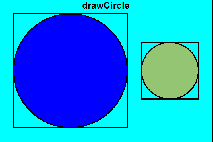
- drawCircle
[Note: the solution for this function is provided for you as an example. See the hw2.py file for details.]
Write the function drawCircle that takes 5 values � a canvas, a left, top, right, and bottom � describing a rectangular region of the canvas, and fills this region with a drawing of a circle. For large areas (>200 pixels wide), the circle should be blue. For smaller areas, it should be pistachio. In either case, it should have a slightly thick black border. Here is a screenshot to help (click on the image to see a larger version):
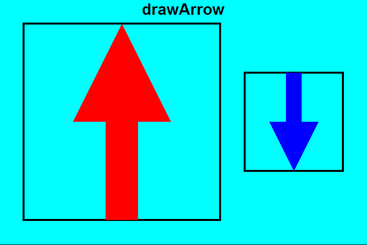
- drawArrow
Write the function drawArrow that takes 5 values � a canvas, a left, top, right, and bottom � describing a rectangular region of the canvas, and fills this region with a drawing of an arrow. For large areas (>200 pixels wide), the arrow should be red and point upwards. For smaller areas, it should be blue and point downwards. Here is a screenshot to help (click on the image to see a larger version):
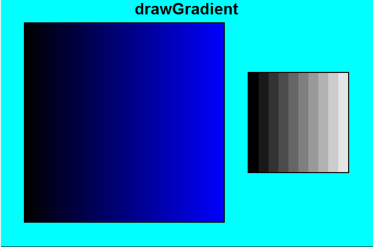
- drawGradient
Write the function drawGradient that takes 5 values � a canvas, a left, top, right, and bottom � describing a rectangular region of the canvas, and fills this region with a drawing of a gradient. This is achieved by drawing a series of rectangles, each a slightly different shade than the previous, uniformly changing from one color on the left to another color on the right. For large areas (>200 pixels wide), the gradient should progress from black to blue using 128 rectangles. For smaller areas, it should progress from black to white, using only 10 rectangles. Here is a screenshot to help (click on the image to see a larger version):
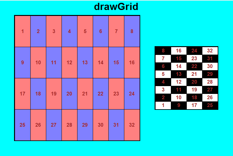
- drawGrid
Write the function drawGrid that takes 5 values � a canvas, a left, top, right, and bottom � describing a rectangular region of the canvas, and fills this region with a drawing of a rectangular grid. For large areas (>200 pixels wide), the grid should have 4 rows and 8 columns, with cells alternating in the shades of red and blue in the image below (or fairly close to them in any case). For smaller areas, the grid should have 8 rows and 4 columns, and the cells should alternate black and white. Also, each cell will be labeled with a number (note that you can provide a number as the text value in create_text). For large areas, the numbers start in the left-top cell and proceed rightwards and then downwards. For small areas, the numbers start in the bottom-left cell and proceed upwards and then rightwards. Here is a screenshot to help (click on the image to see a larger version):
- drawSpiral
Write the function drawSpiral that takes 5 values � a canvas, a left, top, right, and bottom � describing a rectangular region of the canvas, and fills this region with a drawing of an spiral (or really a series of spiral arms). The spiral arms must be created by drawing a series of circles (the only thing drawn in this exercise are small circles). There should be 28 arms, each arm composed of 32 circles. Each arm spirals, or bends, such that the outermost circle in the arm is drawn pi/4 radians (45 degrees) beyond the innermost circle in that same arm. Hint: You will have to use basic trigonometry here! Also, try to make the color gradients work as indicated. Here is a screenshot to help (click on the image to see a larger version):
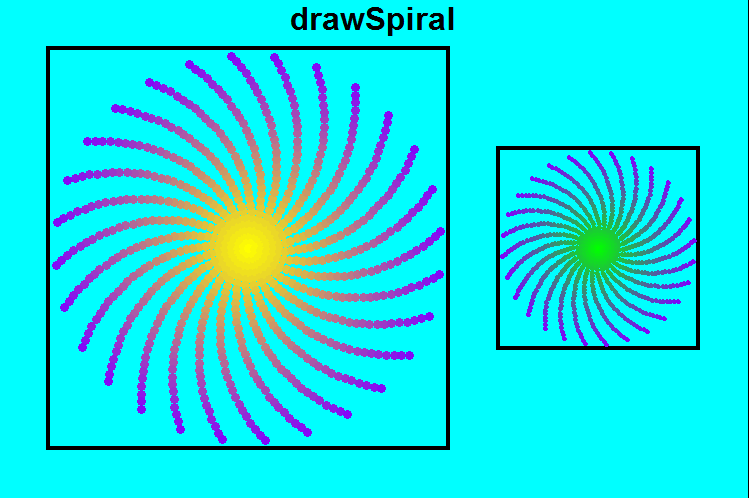
Hint: blue increases from 0 to 255 as the arm spirals outward. Green does the opposite. Only red's behavior changes based on the image size. For the smaller image, red increases from 0 to 128 (not 255). For the larger image, red does something else (what?).
Background: read the first paragraph from the Wikipedia page on happy numbers. After some thought, we see that no matter what number we start with, when we keep replacing the number by the sum of the squares of its digits, we'll always either arrive at 4 (unhappy) or at 1 (happy). With that in mind, we want to write the function nthHappyNumber(n). However, to write that function, we'll first need to write isHappyNumber(n) (right?). And to right that function, we'll first need to write sumOfSquaresOfDigits(n). And that's top-down design! Here we go....
-
sumOfSquaresOfDigits(n)
Write the function sumOfSquaresOfDigits(n) which takes a non-negative integer and returns the sum of the squares of its digits. Here are some test assertions for you:
assert(sumOfSquaresOfDigits(5) == 25) # 5**2 = 25
assert(sumOfSquaresOfDigits(12) == 5) # 1**2 + 2**2 = 1+4 = 5
assert(sumOfSquaresOfDigits(234) == 29) # 2**2 + 3**2 + 4**2 = 4 + 9 + 16 = 29
print "Passed all tests!" - isHappyNumber(n)
Write the function isHappyNumber(n) which takes a possibly-negative integer and returns True if it is happy and False otherwise. Note that all numbers less than 1 are not happy. Here are some test assertions for you:
assert(isHappyNumber(-7) == False)
assert(isHappyNumber(1) == True)
assert(isHappyNumber(2) == False)
assert(isHappyNumber(97) == True)
assert(isHappyNumber(98) == False)
assert(isHappyNumber(404) == True)
assert(isHappyNumber(405) == False)
print "Passed all tests!" - nthHappyNumber(n)
Write the function nthHappyNumber(n) which takes a non-negative integer and returns the nth happy number (where the 0th happy number is 1). Here are some test assertions for you:
assert(nthHappyNumber(0) == 1)
assert(nthHappyNumber(1) == 7)
assert(nthHappyNumber(2) == 10)
assert(nthHappyNumber(3) == 13)
assert(nthHappyNumber(4) == 19)
assert(nthHappyNumber(5) == 23)
assert(nthHappyNumber(6) == 28)
assert(nthHappyNumber(7) == 31)
print "Passed all tests!" - nthHappyPrime(n)
A happy prime is a number that is both happy and prime. Write the function nthHappyPrime(n) which takes a non-negative integer and returns the nth happy prime number (where the 0th happy prime number is 7).
In this exercise, we will observe an amazing property of the prime numbers!
- The Prime Counting Function: pi(n)
Write the function pi(n) (which has nothing much to do with the value "pi", but coincidentally shares its name) that takes an integer n and returns the number of prime numbers less than or equal to n. Here are some test assertions for you:
assert(pi(1) == 0)
assert(pi(2) == 1)
assert(pi(3) == 2)
assert(pi(4) == 2)
assert(pi(5) == 3)
assert(pi(100) == 25) # there are 25 primes in the range [2,100]
print "Passed all tests!"
- The Harmonic Number: h(n)
Write the function h(n) that takes an int n and, if n is positive, returns the sum of the first n terms in the harmonic series: 1/1 + 1/2 + 1/3 + 1/4 + ... If n is non-positive, the function returns 0. Here are some test assertions for you:
assert(almostEquals(h(0),0.0))
assert(almostEquals(h(1),1/1.0 )) # h(1) = 1/1
assert(almostEquals(h(2),1/1.0 + 1/2.0 )) # h(2) = 1/1 + 1/2
assert(almostEquals(h(3),1/1.0 + 1/2.0 + 1/3.0)) # h(3) = 1/1 + 1/2 + 1/3
print "Passed all tests!"
Note: here we use "almostEquals" rather than "==" because this function returns a floating-point number. You should also write almostEquals.
- Using the Harmonic Number to estimate the Prime Counting
Function (Wow!)
Write the function estimatedPi(n) that uses the Harmonic Number function to estimate the Prime Counting Function. Think about it. One counts the number of primes. The other adds the reciprocals of the integers. They seem totally unrelated, but they are in fact very deeply related! In any case, this function takes an integer n and if it is greater than 2, returns the value (n / (h(n) - 1.5) ), rounded to the nearest integer (and then cast to an int). If n is 2 or less, the function returns 0. Here are some test assertions for you:
assert(estimatedPi(100) == 27)
print "Passed all tests!"
- Empirical check that this really works:
estimatedPiError
Write the function estimatedPiError that takes an integer n and returns the absolute value of the difference between the value of our estimation computed by estimatedPi(n) and the actual number of primes less than or equal to n as computed by pi(n). If n is 2 or less, then function returns 0. Here is the start of a test function:
assert(estimatedPiError(100) == 2) # pi(100) = 25, estimatedPi(100) = 27
assert(estimatedPiError(200) == 0) # pi(200) = 46, estimatedPi(200) = 46
assert(estimatedPiError(300) == 1) # pi(300) = 62, estimatedPi(300) = 63
assert(estimatedPiError(400) == 1) # pi(400) = 78, estimatedPi(400) = 79
assert(estimatedPiError(500) == 1) # pi(500) = 95, estimatedPi(500) = 94
print "Passed all tests!"
Aside: as you can see, the estimatedPi function is an amazingly accurate estimation of the pi function. For example, the estimatedPi function predicts that there should be 94 prime numbers up to 500, and in fact there are 95 prime numbers in that range. And so we must conclude that there is some kind of very deep relationship between the sum of the reciprocals of the integers (1/1 + 1/2 + ...) and the number of prime numbers. This relationship has been explored in great detail by many mathematicians over the past few hundred years, with some of the most important results in modern mathematics relating to it.